DOI: 10.5281/zenodo.1492936

Note

A description of the algorithm to calculate a model of the true sky and forward model atmospheric effects to create matched templates.

1 Introduction¶

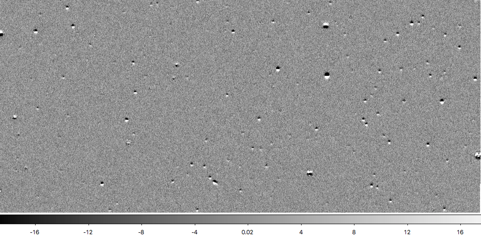
_images/StarFast_1.3_airmass_10deg_diff.png

Figure 1 A difference of two simulated g-band images, observed at elevation angles 10 degrees apart, with no PSF matching to show the dipoles characteristic of mis-subtraction.

Differential Chromatic Refraction (DCR) stretches sources along the zenith direction, so that the sources appear to shift position and the PSF elongates. If all sources had the same spectrum we could correct for the elongation of the PSF with standard PSF-matching tools. In practice, treating DCR in this way can reduce the severity of most of the dipoles in a difference image, since many sources have roughly the same spectrum, but it will make others worse when they don’t match the set selected for calibration. In Figure 1 most of the dipoles point in the same direction since the majority of sources in the simulation have similar (though not identical) spectra, but there are clearly several sources with different spectra where the diploes point in the opposite direction. These differences can’t be accounted for simply with a spatially-varying PSF matching kernel, because the distribution of sources with different spectra is not a simple spatially-varying function; a quasar may be surrounded by a very red galaxy, or a cool, red, star may appear in front of a cluster of young hot stars.

Fundamentally, the problem with correcting DCR through any type of astrometric calibration or PSF matching is that a given pixel of a CCD collects photons from a different solid angle of the sky, and that solid angle depends on wavelength and the observing conditions. Coadding or differencing two images taken under different conditions mixes flux from (slightly) different directions in every pixel, and if the conditions are different enough the quality of the images will degrade (see Figure 3 below for an estimate). Instead, we must use our knowledge of DCR to build deep estimates of the un-refracted sky at sub-filter wavelength resolution, and forward model template images to use for image differencing.

Below, I will first briefly discuss Differential Chromatic Refraction (DCR) in the context of optical telescopes, and LSST in particular. Next I describe my DCR iterative forward modeling approach for solving DCR with software, including the Mathematical framework, Implementation, Examples with simulated images, and Examples with DECam images. I wrap up with a discussion of The DCR Sky Model, a new data product made possible by this approach that allows me to recover Simulated source spectra.

1.1 The origins of Differential Chromatic Refraction¶

As with any medium, light entering Earth’s atmosphere will refract. If the incident light arrives from any direction other than straight overhead, then refraction will bend its path towards an observer such that it appears to come from a location closer to zenith (see Figure 2). While the bulk refraction is easily corrected during astrometric calibration, the index of refraction increases for bluer light and leads to an angular refraction that is wavelength-dependent. Since optical telescopes have a finite bandwidth, this means that a point-like source will get smeared along the direction towards zenith, possibly across multiple pixels. In Figure 3, I calculate the absolute worst case DCR in each of the LSST bands by calculating the difference in refraction for two laser beams of light from the same position but each tuned to one of the extreme wavelengths of the filter. The DCR in this scenario is far more severe than a realistic source spectrum, but it illustrates how the effect will scale with wavelength and zenith angle. Please see Appendix: Refraction calculation for details on the calculation of refraction used throughout this note.

$_images/refraction.gif$

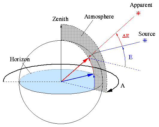
Figure 2 Light incident from a source outside the Earth’s atmosphere refracts and it’s path bends towards zenith. To an observer on Earth, the source appears to be at a higher elevation angle $\Delta E$ than it truly is. For a quick and dirty approximation, $\Delta E$ (in arcseconds) $\sim 90 - E$ (in degrees) = zenith angle. (Image credit: Martin Shepherd, Caltech)

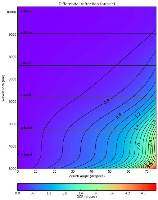
Figure 3 Calculation of the maximum DCR in each of the LSST filters, as a function of zenith angle.

2 DCR iterative forward modeling¶

Because refraction is wavelength-dependent (11), the smearing of astronomical sources will depend on their intrinsic spectrum. In practice, this appears as an elongation of the measured PSF in an image, and a jitter in the source location leading to mis-subtractions in image differencing when looking for transient or variable sources. This effect can be properly corrected when designing a telescope by incorporating an atmospheric dispersion corrector (ADC) in the optical path in front of the detector, but it cannot be removed in software once the photons have been collected. Instead, we can mitigate the effect by building DCR-matched template images for subtraction, and use our knowledge of DCR to build a deep model of the sky from a collection of images taken under a range of observing conditions.

In the sections below, I begin by describing the notation and mathematical framework I will use to solve the problem. I will then lay out the details of my particular implementation of the algorithm, along with a brief discussion of approaches that I have not implemented but might be of interest in the future. Finally, I will give examples using data simulated using StarFast, as well as images from the DECam HiTS survey.

2.1 Mathematical framework¶

The point-spread function (PSF) of a point-like source is a combination of many effects arising from the telescope and its environment. In this note, I will assume that all instrumental effects have been properly measured and accounted for, though this is of course a simplification. Even without instrumental effects, though, we still have the atmosphere to contend with. Turbluence in the atmosphere leads to a blurring of images (seeing), and the severity can vary significantly between nights, or even over the same night. In my initial implementation I will ignore the effect of variable seeing, and use only observations with comparable PSFs, but in order to make full use of all the data available it will have to be addressed in the future (see Extension to variable seeing). Thus, for this initial investigation I will assume that the only effect that changes the shape of the PSF over a set of observations is DCR.

Figure 4 below illustrates the approach of this algorithm. Since DCR arises from the change in the index of refraction of the atmosphere across a filter bandpass, if we can build a model sky in smaller sub-bands the effect is greatly reduced. Further, if DCR is the only effect on the PSF, then we can construct these sub-band models with a small enough bandwidth such that the model to be the same for all observations regardless of airmass and parallactic angle, except for a bulk shift of the entire image. We only measure the combined image from all sub-bands, however, so those shifted sub-band images must be added together, which results in an apparent elongation of the PSF.

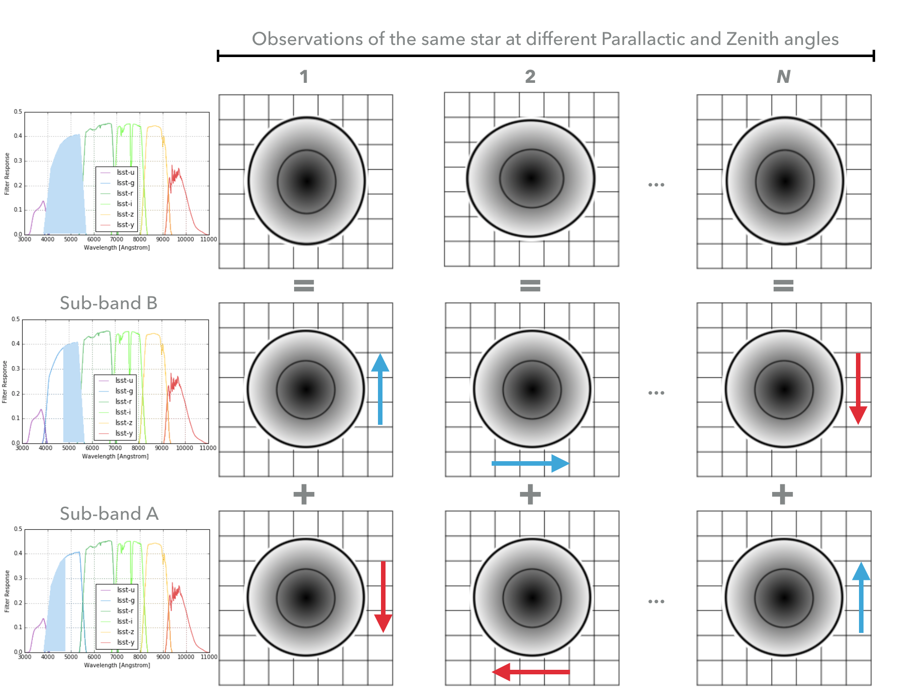
Figure 4 A star observed at different parallactic and zenith angles may appear slightly elongated in the zenith direction, but this is due to DCR. If the full filter were split into two sub-bands (here A and B), the star would appear round(er) but shifted slightly from the position measured across the full band. If we assume that the ‘true’ image within each sub-band does not change, then the changing elongation in the N observed images along the zenith direction can be attributed to these shifts, which we can calculate with (11).

2.1.1 Notation¶

I will use matrix notation throughout this note, with vectors written as lower case letters and 2D matrices written as upper case letters. In this context, images are written as vectors, with all of the pixel values unwrapped. To emphasize this point, I have added arrows over the vectors, though these don’t convey any additional meaning. Image data is written as $\overrightarrow{s_i}$, where the subscript $i$ loops over the input images, while model data is written as $\overrightarrow{y_\alpha}$ with the subscript $\alpha$ looping over sub-bands. While it is often convenient for $\overrightarrow{y_\alpha}$ to have the same resolution and overall pixelization as $\overrightarrow{s_i}$, in general even a non-gridded pixelization such as HEALPix could be used.

The matrix $B_{i\alpha}$ encodes the transformation due to DCR of model plane $\alpha$ to image $i$, and the reverse transformation is written as $B_{\alpha i}^\star$. Since the sub-bands have a narrow bandwidth (but see Finite bandwidth considerations below), the effect of DCR is a uniform shift of all pixels, so:

(1)¶\[B_{\alpha i}^\star B_{i\alpha} = \mathbb{1}\]

Finally, the measured PSF of each image $i$ is given by $Q^{(i)}$, which is a matrix that does not change the size of the image. Or, to put it in more familiar terms, it represents the convolution of any given image with the measured PSF of image $i$. Ignoring effects such as von Karmen turbulence that may lead to a wavelength-dependent PSF size, one fiducial PSF is used for all models without any index: $P$.

2.1.2 Iterative solution derivation¶

The image $\overrightarrow{s_i}$ is the sum of all of the sub-band models (see Figure 4), each shifted by the appropriate amount of DCR relative to the effective wavelength of the full filter from (12):

(2)¶\[ \sum_\alpha B_{i\alpha} \overrightarrow{y_\alpha} = \overrightarrow{s_i}\]

Applying the reverse shift for one sub-band $\gamma$, we can re-write (2) as:

(3)¶\[ \overrightarrow{y_\gamma} = B_{\gamma i}^\star \overrightarrow{s_i} - B_{\gamma i}^\star \sum_{\alpha \neq \gamma} B_{i\alpha} \overrightarrow{y_\alpha}\]

While this may not at first appear to help, we can now solve this problem iteratively. In each iteration, we can solve for a new set of sub-band models $\overrightarrow{y_\gamma}$ using the solutions from the last iteration as fixed input. I will discuss the solutions $\overrightarrow{y_\gamma}$ in a later section, The DCR Sky Model.

Once we have a set of model $\overrightarrow{y_\gamma}$, we can use that to predict the template for a future observation $k$:

(4)¶\[ \parallel \overrightarrow{s_k}\!\!\parallel = \sum_\alpha B_{k\alpha} \overrightarrow{y_\alpha}\]

2.1.3 Finite bandwidth considerations¶

When using three sub-bands for the DCR model the approximation that there is negligible DCR within a sub-band will break down for high airmass observations in the LSST g- or u-band. For example, the differential refraction between 420nm and 460nm under typical observing conditions and at airmass 1.3 is 0.27 arcseconds, or about one LSST pixel. With that amount of variation across a sub-band we clearly cannot expect the simple shift of (2) to work for both low and high airmass observations. One option would be to increase the number of sub-bands of the model, but this introduces additional degrees of freedom that may not be well constrained if we have only a few high airmass observations. Another option would be to exclude high airmass observations, but that would be very unfortunate because the large lever arm of DCR in those observations has the potential to better constrain the model (note that we could still build DCR-matched templates for high airmass observations, even if they are not used to calculate the model). Instead, we can modify $B_{i\alpha}$ to include the effective smearing caused by finite bandwidth:

(5)¶\[ {B}'_{i\alpha} = \int_{\alpha_0}^{\alpha_1} f(\lambda)B_{i\lambda}\mathrm{d}\lambda\]

And (2) becomes:

(6)¶\[ \sum_\alpha {B}'_{i\alpha} \overrightarrow{y_\alpha} = \overrightarrow{s_i}\]

This transformation is the integral of the simple shift $B_{i\alpha}$ across the sub-band, optionally weighted by the filter profile $f(\lambda)$. The identity (1) no longer holds, so we must either accept an approximation or attempt a deconvolution to obtain a modified (3). We have studiously avoided performing any outright deconvolutions, so in my implementation I instead neglect finite bandwidth effects in the reverse transformation and set ${B'}_{i\alpha}^\star = {B}_{i\alpha}^\star$. Now (3) becomes:

(7)¶\[ \overrightarrow{y_\gamma} = B_{\gamma i}^\star \overrightarrow{s_i} - B_{\gamma i}^\star \sum_{\alpha \neq \gamma} {B}'_{i\alpha} \overrightarrow{y_\alpha}\]

And new DCR-matched template images are calculated from the resulting model with:

(8)¶\[ \parallel \overrightarrow{s_k}\!\!\parallel = \sum_\alpha {B}'_{k\alpha} \overrightarrow{y_\alpha}\]

While the above approximations may be unnecessary for low airmass observations, they are also not hurt by making it. It is possible to use equations (2) - (4) for observations where the DCR within sub-bands is small and equations (6) - (8) otherwise, but since the approximation improves as the amount of DCR across a sub-band decreases it seems safe to use for all observations. We may still end up wishing to use the simple shift for low airmass observations if there is a performance difference, however.

2.1.4 Extension to variable seeing¶

While not implemented yet, there is a fairly clear path forward to extend the iterative solution from (3) to the case where additional effects beyond DCR introduce changes to the PSF Variable seeing is the primary concern in this case, but in principle instrumental and other effects could be accounted for in this manner as well.

Now, we need to convolve the model with the measured PSF of the image $Q^{(i)}$, and convolve the image with the fiducial PSF used for the model $P$. This modifies (2) above:

(9)¶\[\sum_\alpha B_{i\alpha} Q^{(i)} \overrightarrow{y_\alpha} = P \overrightarrow{s_i}\]

Now we can once again apply the reverse shift for one sub-band, and re-write (9) as:

(10)¶\[ Q^{(i)}\overrightarrow{y_\gamma} = B_{\gamma i}^\star P \overrightarrow{s_i} - B_{\gamma i}^\star \sum_{\alpha \neq \gamma} B_{i\alpha} Q^{(i)} \overrightarrow{y_\alpha}\]

Unfortunately, we now have improved estimates for $Q^{(i)}\overrightarrow{y_\gamma}$ when what we really want is $y_\gamma$. This problem is identical to the standard problem of image co-addition, however, so at this point we would hook in an existing algorithm for combining images with variable PSFs.

2.2 Implementation¶

There are four main factors to consider when turning (3) into an effective algorithm: what initial solution to use as the starting point for iterations, what conditioning to apply to the new solution found in each iteration, how to detect and down-weight contaminated data, and how to determine when to exit the loop. These factors will each be described in a subsection below.

2.2.1 Finding the initial solution¶

Assuming we have no prior spectral information, the best initial guess is that all sub-bands have the same flux in all pixels. If all model planes are equal at the start, a good guess for the flux distribution within a sub-band is the standard co-add of the input images, divided by the number of model planes being used (since those will be summed). A proper inverse-variance weighting of the input images as part of the coaddition will help make the best estimate, and if there are many input images we could restrict the coaddition to use only those observed near zenith (with negligible DCR). An advantage of selecting the simple coadd as the starting point, is that the solution should immediately converge if the input data exhibits no actual DCR effects, such as redder bands (i-band or redder for LSST) or zenith observations. However, since this image is only the starting point of an iterative process, the final solution should not be sensitive to small errors at this stage.

2.2.2 Conditioning the iterative solution¶

A common failure mode of iterative forward modeling algorithms is oscillating solutions. In these cases, (3) may produce intermediate solutions for $\overrightarrow{y_\gamma}$ with very large amplitude in one iteration, leading to very small amplitude (or negative) solutions in the next iteration, for example. Conditioning of the solution can mitigate this sort of failure, and also help reach convergence faster. Some useful types of conditioning include:

Instead of taking the current solution from (3) directly, use a weighted average of the current and last solutions. This eliminates most instances of oscillating solutions, since it restricts the relative change of the solution between iterations. In the current implementation, the weights are chosen to be the convergence metrics of the two solutions, which allows the overall solution to converge rapidly when possible but cautiously if the solutions oscillate. While the increased rate towards convergence is helpful for well behaved data, the greatest benefit appears when using larger numbers of subfilters. Adding more subfilters beyond the standard three increases the number of degrees of freedom of the problem and increases the susceptibility to unstable and diverging solutions. Using the dynamic weights calculated from the convergence metric allows the solution to make small improvements
Threshold the solutions. Instead of solutions diverging through solutions oscillating between iterations, the solution might ‘oscillate’ between model planes. While it is possible for all of the flux in an image to come from one single model plane, with zero from all others, there are limits. Solutions with more flux near a source in a single plane than the initial coadd are likely to be unphysical, and also likely to be paired with deeply negative pixels in the other planes. Care must be taken to avoid overly strict thresholds that impair convergence (such as applying the preceding test to even noise-like pixels), but reasonable restrictions can eliminate extreme outliers.
Frequency regularization. In addition to comparing the current solution to the last or initial solutions, we could also apply restrictions on variations between model planes. For example, we could calculate the slope (or higher derivatives) of the spectrum for every pixel in the model across the sub-bands, and apply a threshold. Any values deviating more than a set amount from the line (or higher order curve) fit by that slope could be fixed to the fit instead, and minimum and maximum slopes could be set. While I have written an option within the DCR modeling code to enforce this sort of regularization, in practice I have found the additional benefit to be negligible when combined with the preceding forms of conditioning, and leave it turned off by default.

2.2.3 Weighting the input data¶

Weighting of the input data takes two forms: weights that are static properties of the image (such as the variance plane), and dynamic weights that may change between iterations.

Static weights. In most cases the static weights will be just the inverse of the variance planes of the images, and best practice is to maintain separate arrays of inverse-variance weighted image values and the corresponding inverse variance values. All transformations and convolutions are applied to both equally, and the properly weighted solution is the transformed weighted-image sum divided by the transformed weights sum.
Dynamic weights. The simplest form of dynamic weights is a flag, which indicates whether a particular image is to be used in calculating the new solution with (3) or not. If an estimated template is made for each image using the new solution and equation (4), then those templates should become a better fit to the images with every iteration. While it is possible to have a catastrophic failure where the model performs worse for all images, it might also improve for most and degrade for a few. For example, if there are astrometric errors for one image, the pixel-based model may be misaligned to that image and the subtraction residuals may increase between iterations. In that case, that image would hurt the calculation of the overall model more than the additional data was helping it, and that image should be excluded from the next iteration. However, in case the apparent divergence was a fluke, convergence should still be tested for that image on all subsequent iterations in case the fit improves with a better model. It might be possible to re-calibrate images that are flagged in this way, with the hope that an improved astrometric solution would also improve the fit to the model.

2.2.4 Determining the end condition¶

Iterative forward modeling does not have an end condition that can be predetermined, and without setting a limit it would run indefinitely. Possible end conditions include:

Fixed time / number of iterations. The simplest option is to set an upper bound on the number of iterations, to ensure that the loop does exit within a finite time. However, the limit should be set high enough that it does not get hit in typical useage.
Test for convergence. There are two types of tests that check for convergence; one that is fast and one that is accurate. The fast check simply compares the rate of change of the solution, and if the difference between the new and the last solution is less than a specified threshold fraction of the average of the two the solution has converged. The accurate check, on the other hand, creates a template for each image using (4), and calculates a convergence metric from the difference of each image from its template. Once the convergence metric changes by less than a specified level between iterations we can safely exit the loop since additional iterations will provide insignificant improvement. This is slower since templates must be created for each image, for every iteration, but that has the advantage of allowing convergence to be checked for each individual image at no extra cost (see “Dynamic weights” above). If the extra computational cost is not considered prohibitive, then the second test of convergence is far superior, since it is more accurate and enables additional tests and weighting. The level of convergence reached will clearly impact the quality of the results; see Simulated source spectra below for more analysis.
Test for divergence. If a template is made for testing convergence, we should naturally test also for divergence. If the convergence metric actually degrades with a new iteration, that is a clear sign that some feature of the image is being modeled incorrectly and more iterations will only exacerbate the problem. One special case is if only some of the images degrade, because it is possible that they contain astrometric or other errors, and we could choose to continue with those observations flagged (see “Dynamic weights” above). Otherwise, it is safest to exit immediately and discard the solution from the current iteration, using the last solution from before it started to diverge instead.
- One possible modification is to calculate a spatially-varying convergence metric, and mask regions that degrade in future iterations. This allows an improved solution to be found even if one very bright feature (such as an improperly-masked saturated star or cosmic ray) is modeled incorrectly.

Note that if a convergence test is used, it should only be allowed to exit the loop after a minimum number of iterations have passed. It will depend on how the convergence metric is calculated and the choice of initial solution, but the first iteration can show a slight degradation of convergence.

2.3 Examples with simulated images¶

To test the above algorithm, I first ran it on images simulated using StarFast. As shown in Figure 5 below, these images contain a moderately crowded field of stars (no galaxies) with Kolmogorov double-gaussian PSFs, realistic SEDs, photon shot noise, and no other effects other than DCR. In this example, the model is built using three frequency planes and eight input simulations of the field, with airmass ranging between 1.0 and 2.0 (not including the simulated observation shown in Figure 5). I use (4) to build a DCR-matched template for the simulated observation (Figure 6), and subtract this template to make the difference image (Figure 7). For comparison, in Figure 8 I subtract a second simulated image generated with the same field 10 degrees closer to zenith. Note that the noise in Figure 7 is $\sim \sqrt{2}$ lower than in Figure 8, because the template is a form of coadded image with significantly lower noise than an individual exposure.

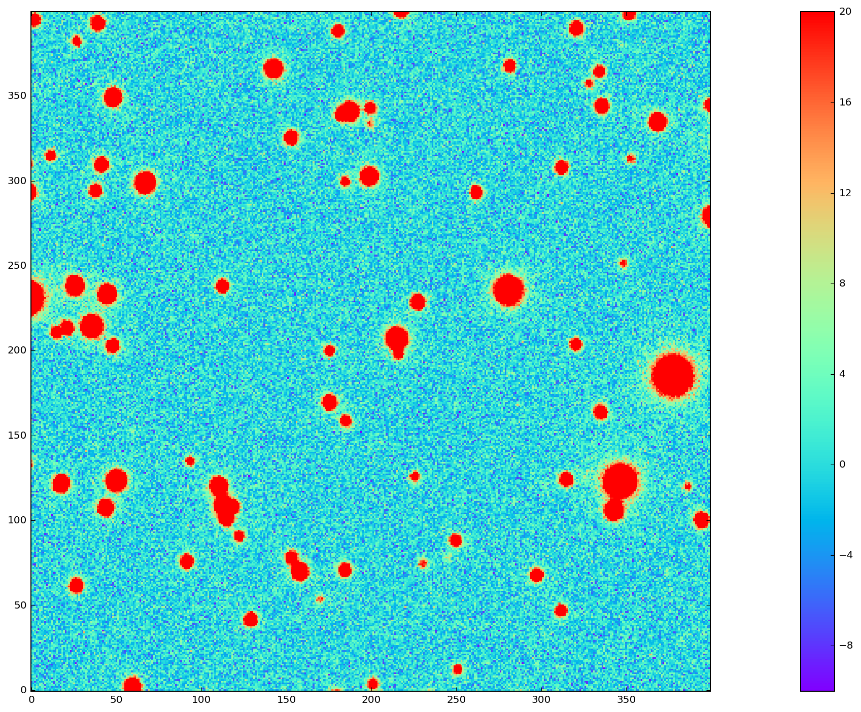
Figure 5 Simulated g-band image with airmass 1.3

_images/simulated_image_108_template.png

Figure 6 The DCR-matched template for the simulated image in Figure 5. Because the template consists of a coaddition of multiple images, the noise is significantly reduced.

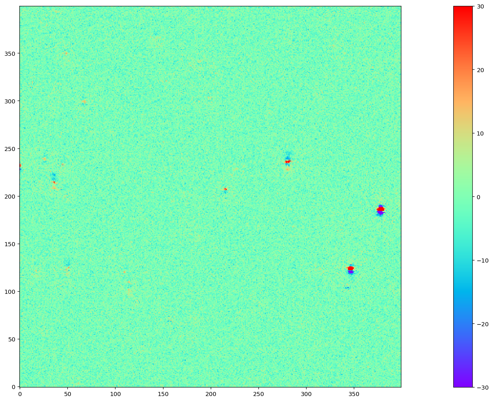
_images/simulated_image_108_template_difference.png

Figure 7 Image difference of the simulated image Figure 5 with its template from Figure 6. The image difference is taken as a direct pixel subtraction, rather than an Alard & Lupton or ZOGY style subtraction. While those more sophisticated styles of subtraction are used in production, here the emphasis is on comparing the raw differences, before PSF matching or other corrections.

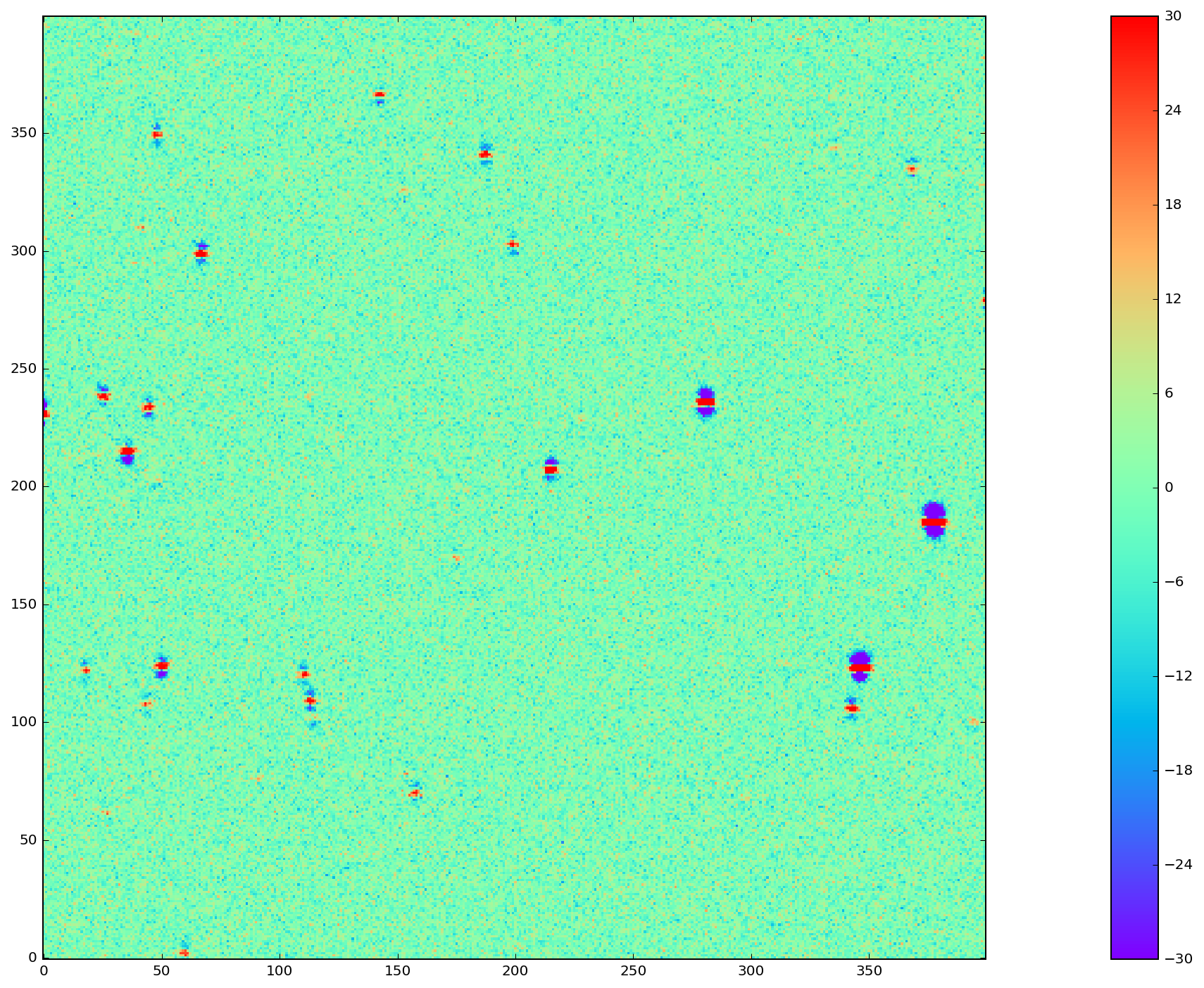
_images/simulated_image_108_112_difference.png

Figure 8 Image difference of Figure 5 with another simulation of the same field 10 degrees closer to zenith (airmass 1.22). As in Figure 7 above, this image difference is a direct pixel subtraction and not an Alard & Lupton or ZOGY style subtraction. By eye, there are significantly more mis-subtractions than when using the matched template (Figure 7), which results in an increase in the number of false detections. See Figure 9 for a quantitative evaluation of the number of false positives when using different templates for subtraction.

2.3.1 Dipole mitigation¶

A quantitative assessment of the quality of the template from Figure 6 is the number of false detection in the image difference, Figure 7. Since there are no moving or variable sources in these simulated images, any source detected in the image difference is a false detection. From comparing Figure 7 and Figure 8 it is clear by eye that the DCR-matched template produces fewer dipoles, and we can see in Figure 9 that this advantage holds regardless of airmass or elevation angle. The DCR-matched template appears to perform about as well as an exposure taken within 5 degrees of the science image, but recall that the noise - and therefore the detection limit - is higher when using a single image as a template. While the difference images of Figure 7 and Figure 8 above simply performed direct subtraction of the pixels, here I use an Alard & Lupton-style image difference using the LSST software stack to detect sources.

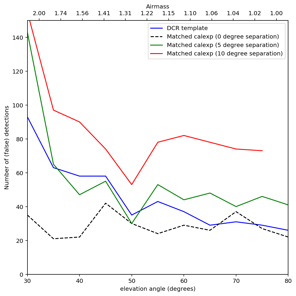
Figure 9 Plot of the number of false detections for simulated images as a function of airmass, for different templates. For the “0 degree separation” difference images (dashed line), the simulated images were re-generated with the same observing conditions but a different realization of the noise. This provides an estimate of the minimum number of false positives that should be expected for these simulations.

2.4 Examples with DECam images¶

For a more rigorous test, I have also built DCR-matched templates for DECam HiTS observations, which were calibrated and provided by Francisco Förster. For these images I used the implementation outlined above using the simplified equation (3), despite the images having variable seeing. Because I have not yet implemented (10) using measured PSFs for each image, I have simply excluded observations with PSF FWHWs greater than 4 pixels (2.5 - 4 pixel widths are common). However, it should be noted that the images with PSFs at the larger end of that range are not as well matched by their templates, so restricting the input images going into the model to those with good seeing may not be sufficient in the future.

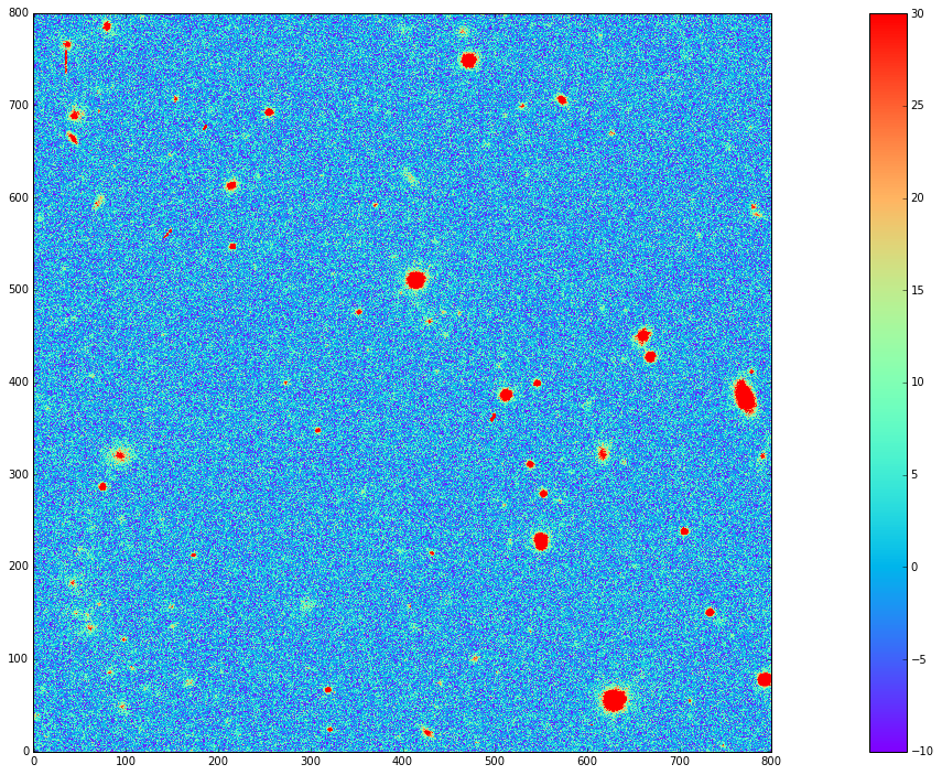
Figure 10 Decam observation 410998, ‘g’-band with airmass 1.33.

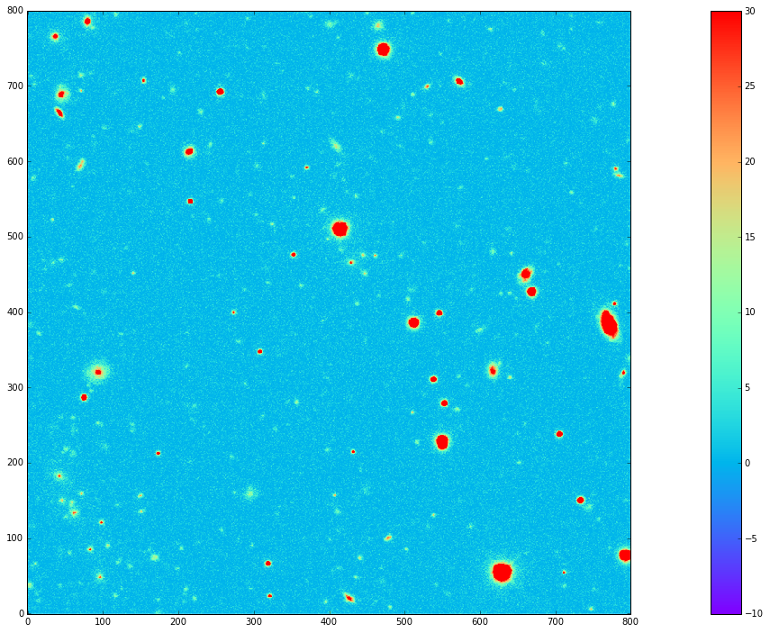
Figure 11 The DCR-matched template for 410998, constructed from 12 observations with airmass ranging between 1.13 and 1.77. Note that the noise level is significantly decreased.

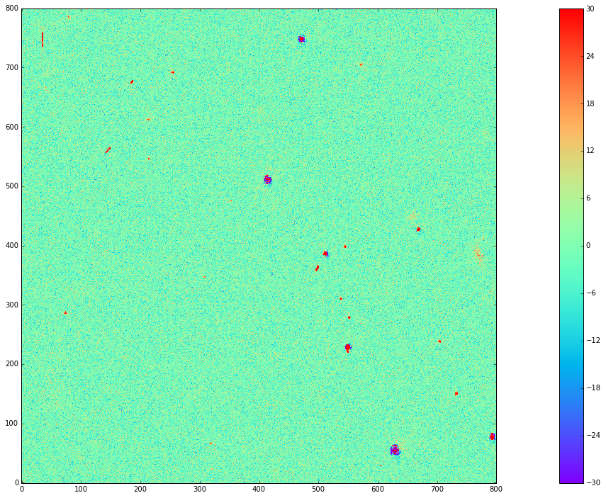
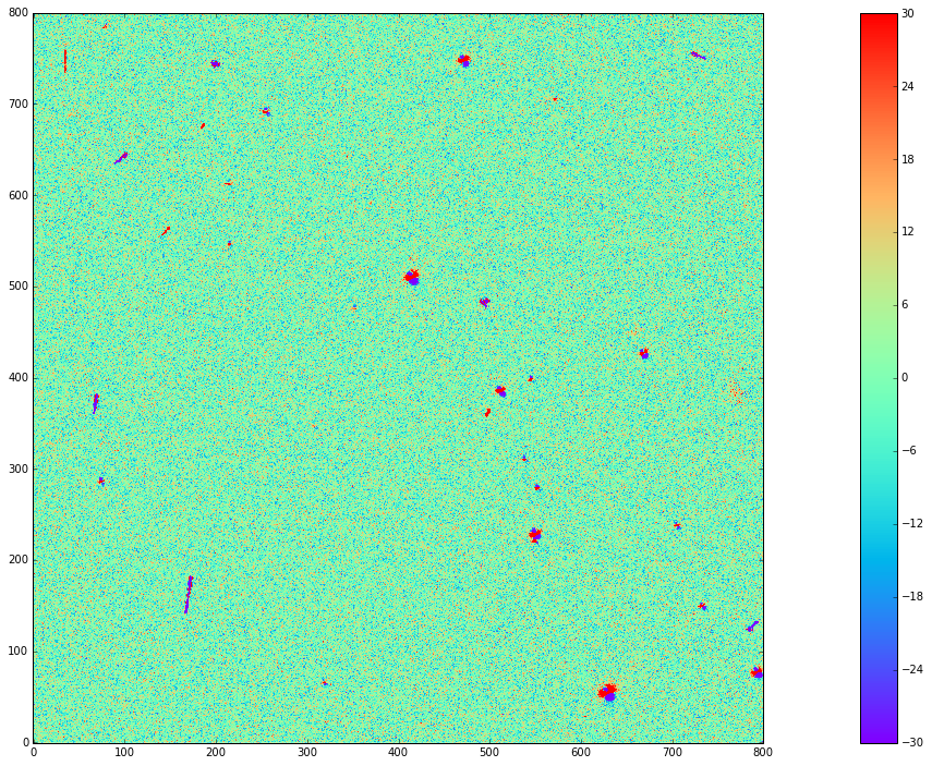
Figure 12 Difference image of Figure 10 - Figure 11.

Figure 13 Image difference of Figure 10 with a second DECam observation taken an hour later and approximately 10 degrees closer to zenith (at airmass 1.23).

From the above images we can make several observations. First is that the DCR-matched template in Figure 12 performs at least as well as a well-matched reference image taken within an hour and 10 degrees of our science image (Figure 13). The DCR-matched template, however, has significantly reduced noise and artifacts (such as cosmic rays), since we are able to coadd 12 observations because we are not constrained by needing to match observing conditions. Thus, a DCR-matched template calculated at zenith should provide the cleanest and deepest estimate of the static sky possible from the LSST survey, since we can coadd all images without sacrificing image quality or resolution.

While constructing the DCR sky model for a full DECam CCD was time consuming on my laptop (taking about 10 minutes on one core), forward modeling a DCR-matched template from the model takes only 1-2 seconds on the same machine. Adding variable the PSFs from (10) will increase the time required to calculate the DCR sky model, but should not increase the time to forward model templates.

3 The DCR Sky Model¶

The DCR sky model $\overrightarrow{y_\alpha}$ from (3) consists of a deep coadd in each subfilter $\alpha$. As with other coadds, the images are defined on instrument-agnostic tracts and patches of the sky, and must be warped to the WCS of the science image after constructing templates with (4). While the sky model was designed for quickly building matched templates for image differencing, it is an interesting data product in its own right. For example, we can run source detection and measurement on each sub-filter image $\overrightarrow{y_\alpha}$ and measure the spectra of sources within a single band. An example visualization of the sub-bands of the DCR sky model is in Figure 14, below, while a more detailed look at spectra is in Simulated source spectra. This view can help identify sources with steep or unusual spectra, such as quasars with high emission in a narrow band, and could be used to help deblending and star-galaxy separation. However, because of the inherent assumption that the true sky is static it cannot estimate the spectrum of transient or variable sources.

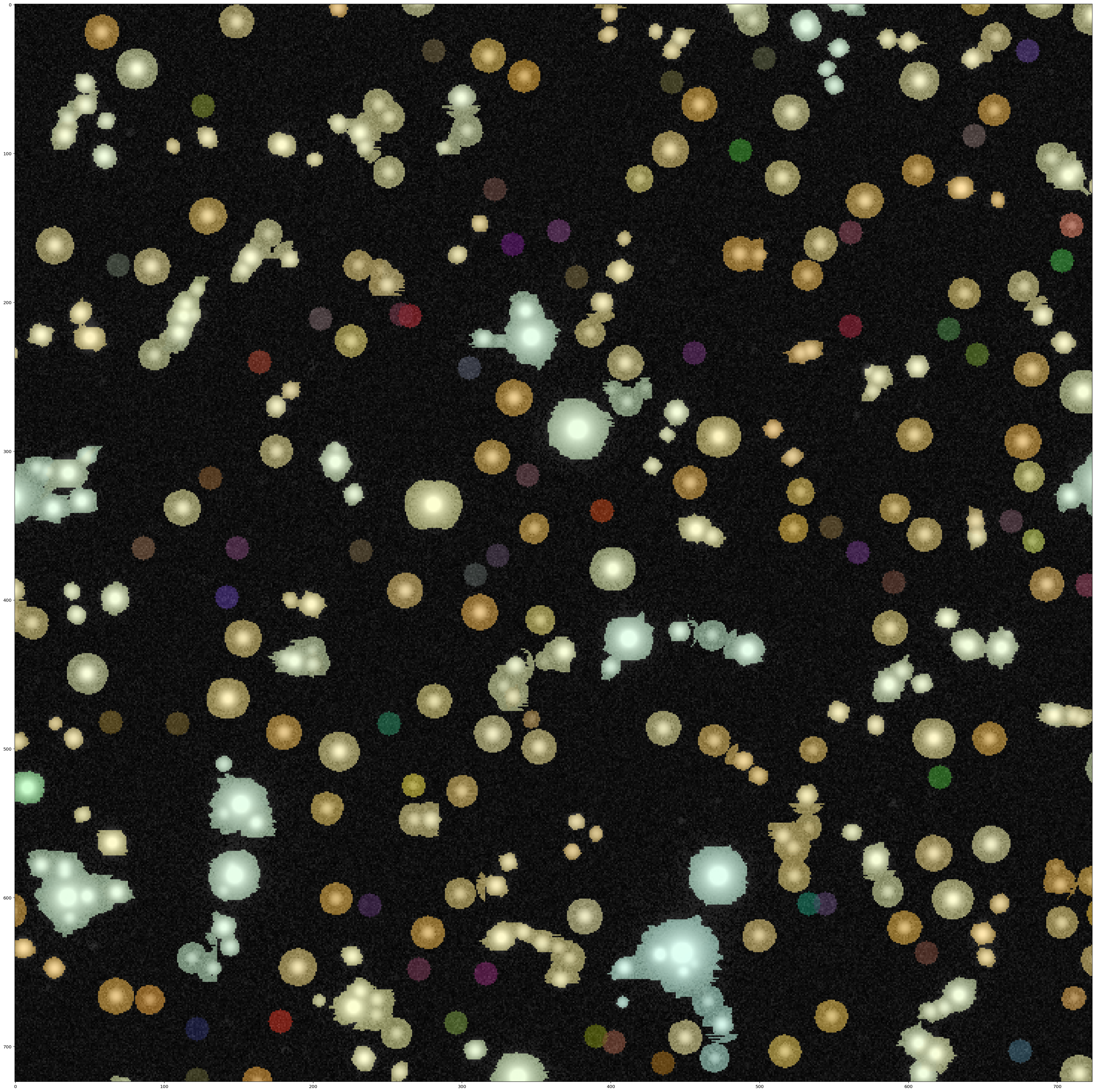
_images/sim_filled_footprints_color2.png

Figure 14 Source measurements in three sub-bands of the DCR sky model are converted to RGB values and used to fill the footprints of detected sources. The combined full-band model is displayed behind the footprint overlay.

3.1 Simulated source spectra¶

As mentioned above, we can look in more detail at the spectra of individual sources. The simulated images contain roughly 2500 stars ranging from type M to type B, with a distribution that follows local abundances. Each star is simulated at high frequency resolution using Kurucz SED profiles and propagated through a model of the LSST g-band filter bandpass, so it is straightforward to compare the measured spectrum of a source to its input spectrum once it is matched. To measure the subfilter source spectra, I run multiband photometry from the LSST multiband processing framework [1] with coaddName=dcr set. This performs source detection on each subfilter coadd image, merges the detections from all subfilters, and performs forced photometry on each. A few example comparison spectra for a range of stellar types are in Figure 15 - Figure 19 below [2].

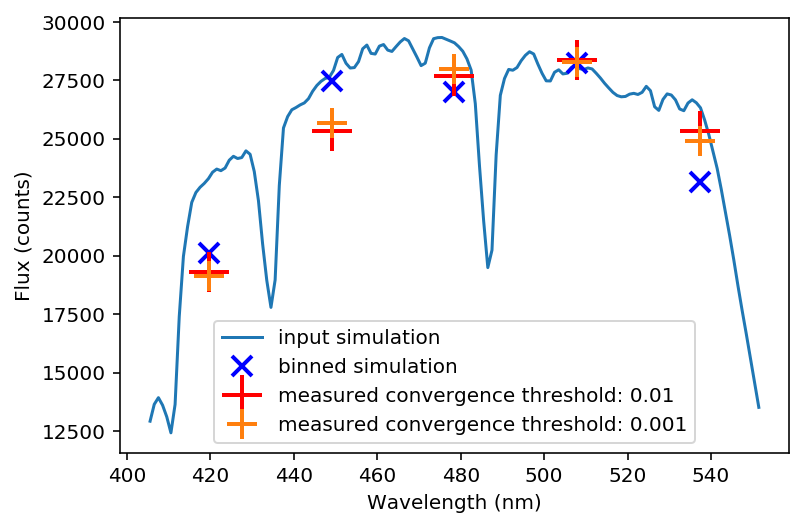
Figure 15 Example input spectrum for a type A star with surface temperature ~8167K (solid blue). The flux measured in each of five sub-bands is marked with a ‘+’, and the average values of the simulated spectrum across each subfilter is marked with a blue ‘x’ for comparison. Two measurements are plotted for each sub-band: the result from ending forward modeling when the convergence metric reached 1% in red, and 0.1% in orange.

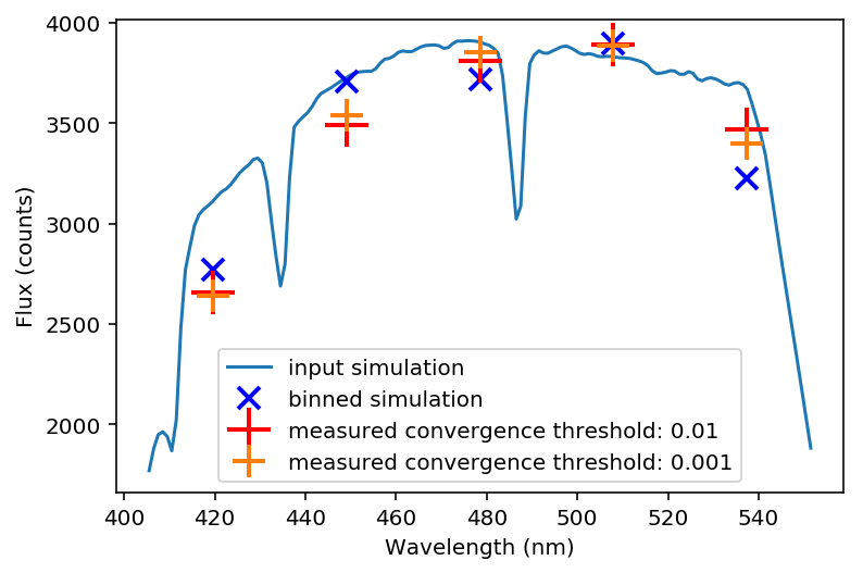
Figure 16 Example input spectrum for a type F star with surface temperature ~6909K (solid blue). The symbols are as Figure 15.

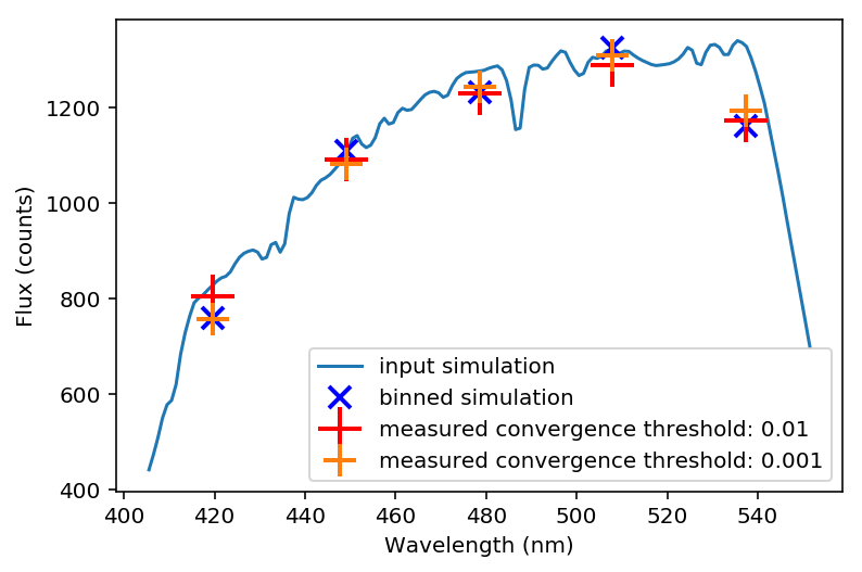
Figure 17 Example input spectrum for a type G star with surface temperature ~5991K (solid blue). The symbols are as Figure 15.

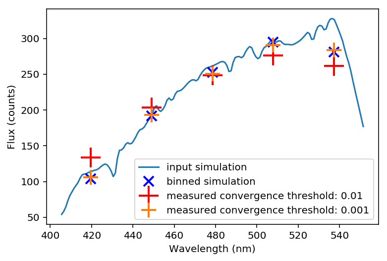
Figure 18 Example input spectrum for a type K star with surface temperature ~5006K (solid blue). The symbols are as Figure 15.

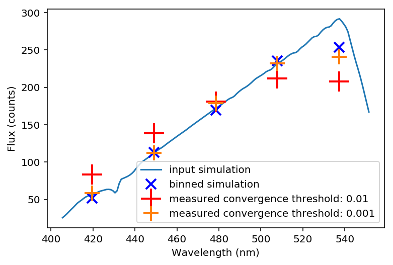
Figure 19 Example input spectrum for a type K star with surface temperature ~3907K (solid blue). The symbols are as Figure 15.

While the above spectra are representative of the typical stars in the simulation, it is helpful to look at the entire set. For this comparison, in Figure 20 below I plot the simulated color between the blue and the red subfilters against the measured color, ignoring the center subfilter. For this example, I let the forward modeling proceed until it reached 1% convergence, which took 8 iterations. While there is a clear correlation between the measured and simulated spectra the slope is clearly off, with the measurements flatter than the simulations. If a 0.1% convergence threshold is used, however, then after 50 iterations the agreement improves (Figure 21). The example spectra in Figure 15 - Figure 19 above used the 0.1% threshold.

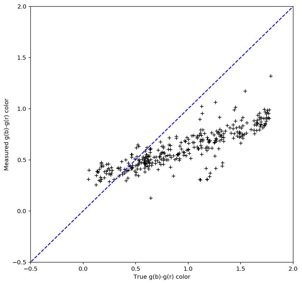
Figure 20 Simulated - measured color of detected sources within g-band with a 1% convergence threshold. Convergence was reached after 8 iterations of forward modeling.

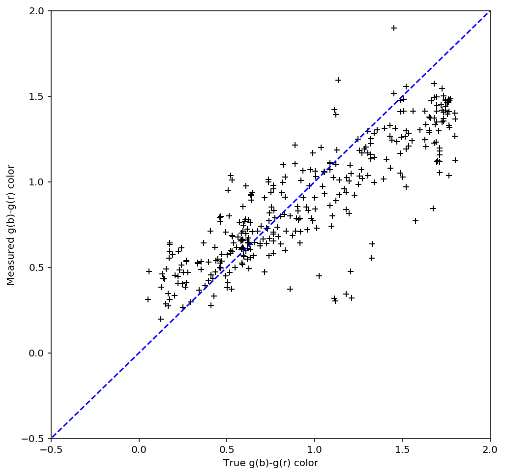
Figure 21 Simulated - measured color of detected sources within g-band with a 0.1% convergence threshold. Convergence was reached after 50 iterations of forward modeling.

[1]	The LSST multiband processing framework used for these examples was version `w_2018_43` of the `lsst_distrib` codebase.

[2]

Previous versions of this document used a prototype implementation of the algorithm to generate the DCR models used for source measurement in Simulated source spectra . A careful reader will note a few differences in the plots in this section: the number of DCR subfilters, and consequently the number of measurements of each spectrum, has been increased from 3 to 5, which is due to improvements in the stability of the algorithm that support higher numbers of subfilters. Additionally, there is now greater scatter in the recovered color vs simulated color plots (Figure 20 and Figure 21). The new implementation includes astrometric calibration, which in the case of simulations introduces slight position errors due to fitting sources affected by DCR.

4 Appendix: Refraction calculation¶

While the true density and index of refraction of air varies significantly with altitude, I will follow [Sto96] in approximating it as a simple exponential profile in density that depends only on measured surface conditions. While this is an approximation, it is reportedly accurate to better than 10 milliarcseconds for observations within 65 degrees of zenith, which should be sufficient for normal LSST operations.

The refraction of monochromatic light is given by

(11)¶\[\begin{split}R(\lambda) &= r_0 n_0(\lambda) \sin z_0 \int_1^{n_0(\lambda)} \frac{dn}{n \left(r^2n^2 -r_0^2n_0(\lambda)^2\sin^2z_0\right)^{1/2}} \nonumber\\ &\simeq \kappa (n_0(\lambda) - 1) (1 - \beta) \tan z_0 - \kappa (1 - n_0(\lambda)) \left(\beta - \frac{n_0(\lambda) - 1}{2}\right) \tan^3z_0\end{split}\]

where $n_0(\lambda)$, $\kappa$, and $\beta$ are given by equations (13), (17), and (18) below. The differential refraction relative to a reference wavelength is simply:

(12)¶\[\Delta R(\lambda) = R(\lambda) - R(\lambda_{ref})\]

The index of refraction as a function of wavelength $\lambda$ (in Angstroms) can be calculated from the relative humidity ($RH$, in percent), surface air temperature ($T$, in Kelvin), and pressure ($P_s$ in millibar):

(13)¶\[\begin{split}n_0( \lambda ) &=\:& 1 + \Delta n_s + \Delta n_w \\ \\ \Delta n_s &=\:& \bigg(2371.34 + \frac{683939.7}{130 -\sigma(\lambda)} + \frac{4547.3}{38.9 - \sigma(\lambda)^2}\bigg) D_s \times 10^{-8} \\ \\ \Delta n_w &=\:& \big(6487.31 + 58.058 \sigma(\lambda)^2 - 0.71150\sigma(\lambda)^4 + 0.08851\sigma(\lambda)^6\big) D_w \times 10^{-8} \\ \\ \sigma(\lambda) &=\:& 10^4/\lambda \;\;\;( \mu m^{-1})\end{split}\]

Where the density factors for water vapor $D_w$ and dry air $D_s$ are given by (14) and (15) (from [Owe67]), and the water vapor pressure $P_w$ is calculated from the relative humidity $RH$ with (16).

(14)¶\[D_w = \bigg[1+P_w (1+3.7\times10^{-4}P_w)\bigg(-2.37321\times 10^{-3} + \frac{2.23366}{T} - \frac{710.792}{T^2} + \frac{7.75141\times 10^4}{T^3}\bigg)\bigg] \frac{P_w}{T}\]

(15)¶\[D_s = \bigg[1 + (P_s - P_w) \bigg( 57.90 \times 10^{-8} - \frac{9.3250\times 10^{-4}}{T} + \frac{0.25844}{T^2}\bigg)\bigg] \frac{P_s - P_w}{T}\]

(16)¶\[P_w = RH\times 10^{-4}\times e^{(77.3450 + 0.0057 T - 7235.0/T)}/T^{8.2}\]

The ratio of local gravity at the observing site to $g= 9.81 m/s^2$ is given by

(17)¶\[ \kappa = g_0/g = 1 + 5.302\times 10^{-3} \sin^2\phi - 5.83\times 10^{-6} \sin^2(2\phi) - 3.15\times 10^{-7} h \label{eqn:kappa}\]

By assuming an exponential density profile for the atmosphere, the ratio $\beta$ of the scale height of the atmosphere to radius of the observing site from the Earth’s core can be approximated by:

(18)¶\[\begin{split}\beta &= \frac{1}{R_\oplus}\int_{0}^\infty \frac{\rho}{\rho_0} dh \nonumber \\ &\simeq \frac{P_s}{\rho_0g_0 R_\oplus} = \frac{k_BT}{m g_0 R_\oplus} \nonumber \\ &= 4.5908\times 10^{-6} T\end{split}\]

where $m$ is the average mass of molecules in the atmosphere, $R_\oplus$ is the radius of the Earth, $k_B$ is the Boltzmann constant, and $g_0$ is the acceleration due to gravity at the Earth’s surface.

5 References¶

[Owe67]

James C. Owens. Optical refractive index of air: dependence on pressure, temperature and composition. Appl. Opt., 6(1):51–59, Jan 1967. http://ao.osa.org/abstract.cfm?URI=ao-6-1-51. URL: http://ao.osa.org/abstract.cfm?URI=ao-6-1-51, doi:10.1364/AO.6.000051.

[Sto96]

Ronald C. Stone. An Accurate Method for Computing Atmospheric Refraction. Publications of the Astronomical Society of the Pacific, 108(729):1051, nov 1996. URL: http://www.jstor.org/stable/10.2307/40680838, doi:10.1086/133831.

DMTN-037: DCR-matched template generation